
The Quintic Root of Hipparchus
UPDATED 22/02/28
Nighttime light pollution is sadly familiar to all of us. While our grandparents and great-grandparents may talk fondly of seeing the Milky Way in their youth, with thousands of stars scattered across the dark summer sky, we are mostly content with seeing a few dozen stars through the never-ending dusk of urban and suburban skies.
As professional lighting designers, we know the solutions. First, we need to limit the amount of light that is uselessly directed or reflected upwards into the night sky from streetlights and outdoor area lighting. Second, we need to minimize the relative amount of blue light generated by the light sources. Third, we should dim or turn off the lighting when it is not needed. Three simple but effective solutions.
The question is, how do we quantify these solutions? What does it mean, for example, to “minimize the relative amount of blue light”? Indeed, how do we even define “blue light?” More important, what is the result of doing so? Given two light sources – for example, 2700K and 3000K LED streetlights – which is the better choice in terms of reducing nighttime skyglow? Is it even worth worrying about the difference?
What we are really asking here is, what is the relationship between the spectral power distribution (SPD) of a light source and its contribution to nighttime sky glow? If we know the answer to this question, we can make quantitative and hence informed judgements when choosing exterior luminaires for street and area lighting.
What we need is (yet another) lighting design metric.
Correlated Color Temperature
At present, we are advised to simply choose luminaires with low CCTs. Indeed, the International Dark-Sky Association mandates luminaires with CCTs of 3000K or lower for its IDA Fixture Seal of Approval program, and is recommending luminaires with CCTs of no more than 2200K. Unpublished studies of over one thousand commercial LEDs have shown a strong correlation between CCT and the relative amount of blue light, so this is arguably a reasonable approach.
The problem however is that the 3000K limit is entirely prescriptive. If there is an application where a higher CCT is desired or even necessary, there is no opportunity for lighting designers to make a design decision based on factual information.
Other Metrics
Several other design metrics have been proposed, all with various shortcomings. For example, the scotopic-photopic ratio (S/P) may provide a reasonable indication of the relative amount of blue light in an SPD, but it is based solely on the human visual system. It may be useful for ranking light sources according to their relative blue light content, but it is not a quantitative measure.
Another approach is to specify an arbitrary division between blue and “not blue” light (typically 500 nm or 520 nm) and calculate the relative blue light content directly from the SPD. This approach is based solely on the SPD, with no reference to the human visual system or the illuminated environment. As such, it yields a metric that is useful only for ranking light sources according to their relative blue light content; it is not a quantitative measure.
What is needed is a metric that takes into account:
- Spectral power distribution;
- Photopic vision;
- Scotopic vision; and
- Atmospheric scattering
as these are the components of what we perceive as artificial sky glow and hence light pollution.
Ancient History
To develop a quantitative light pollution metric, we need to start at the desired end result and work backwards. To do so, we need to go back over two millennia to the time of Hipparchus of Nicaea (190 – c. 120 BC). Hipparchus was a Greek astronomer, geographer, and mathematician. Considered possibly the greatest astronomer of antiquity, he compiled the first comprehensive star catalog in the Western world. While this catalog has been lost to the mists of time, it likely contained at least 850 stars. More important for our needs, he is conjectured to have ranked the apparent magnitude (visual brightness) of stars on a scale of 1 (brightest) to 6 (faintest).
Moving forward in time some two thousand years, an English astronomer named Norman Robert Pogson was working at the Madras observatory in India when in 1856, he decided to place Hipparchus’s apparent magnitude scale on a firm mathematical footing.
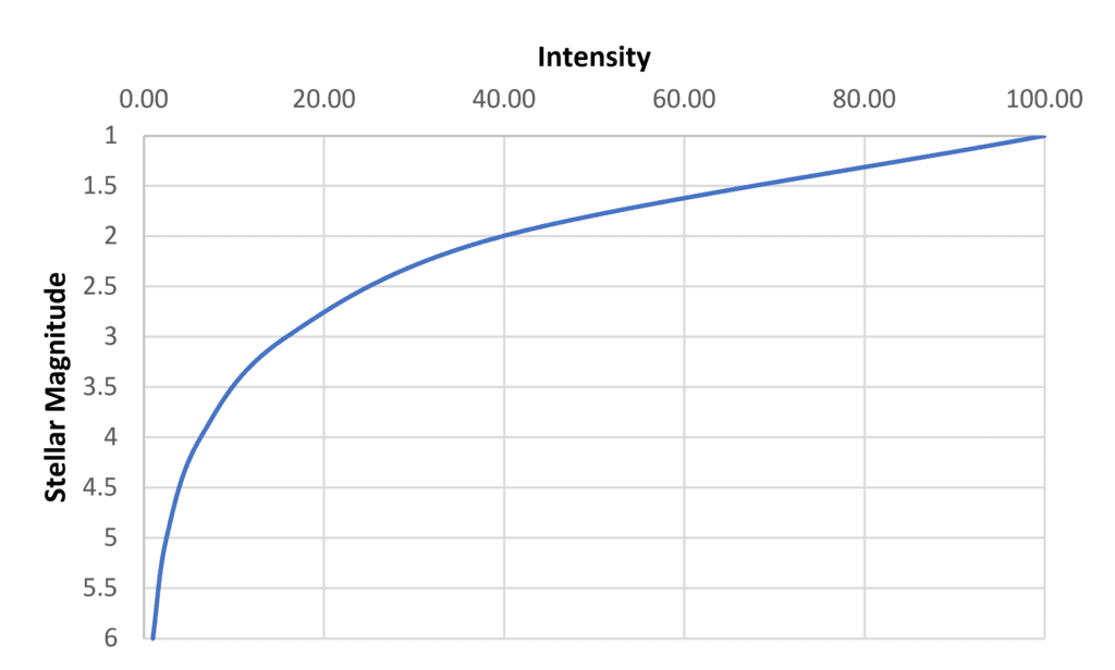
Noting that the perceived brightness of a point source of light varies approximately logarithmically with intensity, and that the photometric intensity of a first-magnitude star was approximately one hundred times that of a sixth-magnitude star, he proposed that a difference of one magnitude be equal to 1001/5, or about 2.512 (Pogson’s Ratio), in intensity (FIG. 2). Hence the fifth, or “quintic,” root of Hipparchus.
Hipparchus’ apparent magnitude scale is open-ended – the magnitude of the brightest star Sirius is -1.46 (note the negative value), while large amateur telescopes are capable of detecting stars as faint as 16 on exceptionally clear nights. The number of visible stars with a given magnitude or brighter varies with latitude and season, but Table 1 provides a reasonable average estimate.
| Apparent Magnitude | Number of Stars |
| 1 | 15 |
| 2 | 48 |
| 3 | 171 |
| 4 | 513 |
| 5 | 1602 |
| 6 | 4800 |
The point here is not the exact number of stars that are visible, but that the number depends on the sky brightness (or more properly, sky luminance). The faintest stars that can be seen on an exceptionally clear and dark night with fully dark-adapted eyes (i.e., scotopic vision) is about magnitude 6. In an area with a lot of light pollution, the limiting magnitude due to artificial sky glow can be as low as 2 or 3.
This is something that elementary school children can explain to their great-grandparents: the more light pollution there is, the fewer stars that can be seen. If we can calculate the difference in limiting magnitude due to light sources with different SPDs, all other factors being equal, we will have a quantitative light pollution metric.
Typical Outdoor Light Sources
Spectral power distributions for both luminaires and light sources (lamps and LED modules) are almost impossible to obtain from their manufacturers. Fortunately, CIE 015:2018, Colorimetry, Fourth Edition (CIE 2018) publishes the SPDs of two typical high-pressure sodium lamps, three metal halide lamps, and four light-emitting diodes that are representative of the light sources typically used for outdoor lighting applications.
Table 2 enumerates these light sources, along with the SPDs of anonymous products representing 2200K white light, phosphor-coated amber, and narrowband (quasimonochromatic) amber LEDs that are recommended by the International Dark-Sky Association.
| Light Source | Description |
| CIE HP1 | 1950K HPS |
| CIE HP2 | 2500K HPS |
| CIE HP3 | 3100K MH |
| CIE HP4 | 4000K MH |
| CIE HP5 | 4000K MH |
| CIE B1 | 2700K LED |
| CIE B2 | 3000K LED |
| CIE B3 | 4000K LED |
| CIE B4 | 5000K LED |
| Generic 2200K | 2200K LED |
| Generic PC Amber | PC amber LED |
| Generic Amber | Narrowband amber LED |
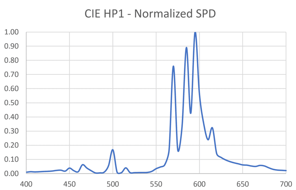
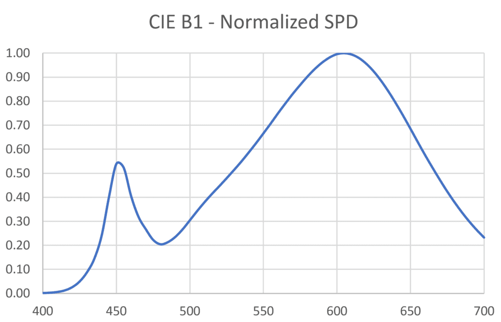
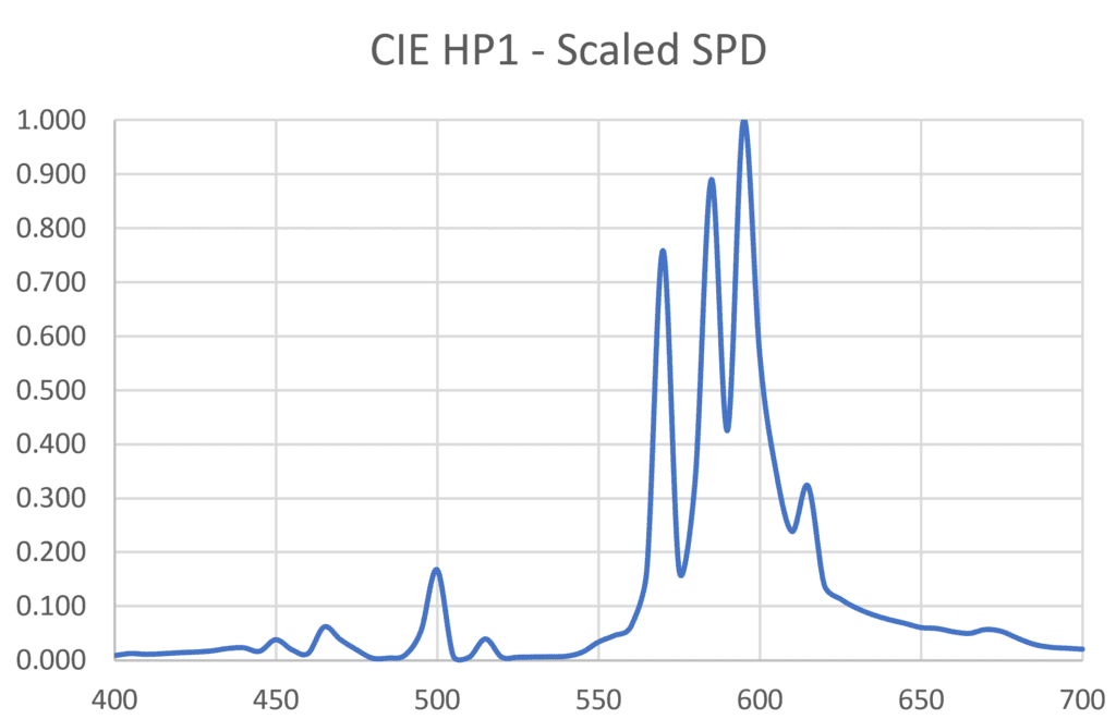
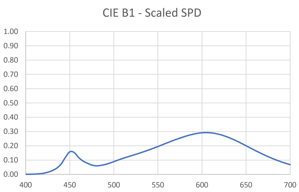
To simplify matters, we can assume that two or more different light sources have the same luminous intensity distribution and luminous flux output; the only difference is their spectral power distribution. Given this, we begin by choosing two light sources, say CIE HP1 and CIE B1, for comparison, with their normalized SPDs as shown in Figure 3. The physical sources they represent – a high-pressure sodium lamp and a single LED – will obviously have different luminous flux outputs. We therefore need to scale these SPDs such that they represent the same luminous flux.
Photopic Vision
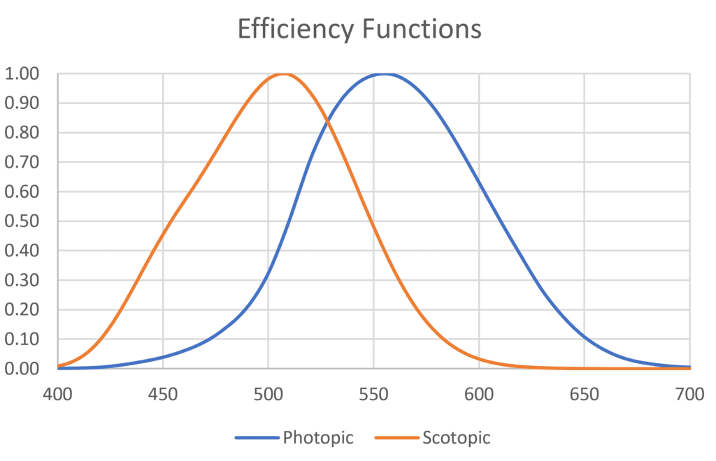
Lighting design for roadway and area lighting applications is typically based on photopic illuminance values. If we multiply each tabulated value of the light sources SPDs on a per-wavelength basis by the corresponding value of the photopic efficiency function V(λ) of Figure 4, we can sum the resultant values and multiply this sum by a constant to obtain the lumens emitted by the light source.
The constant is not important here, as we only need to ensure both light sources are emitting the same number of lumens (i.e., luminous flux). In the example given here, the sum for the CIE HP1 lamp is 4.373, while the sum for the CIE B1 source is 14.969. If we nominate CIE HP1 as our baseline light source, we then need to scale the CIE B1 SPD by 4.373 / 14.969 = 0.292. The scaled SPDs are shown in Figure 5.
Atmospheric Scattering
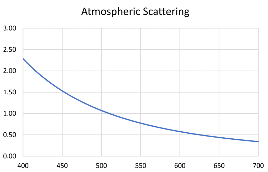
Our atmosphere preferentially scatters blue light, which is why the sky is blue on a clear day. This is caused by Rayleigh scattering from nitrogen and oxygen molecules, but there is also Mie scattering, which is caused by aerosols such as water droplets, dust and smog. Mie scattering is wavelength-independent, which is why fog and clouds, for example, are gray.
At a distance of 80 kilometers (50 miles) from a city center, both Rayleigh and Mie scattering contribute to sky glow that is caused by electric lighting. A study by Aubé (2015) provides an approximate scattering function:
S = (550/λ)2.7
where λ is the wavelength in nanometers. This function (which assumes that we are looking straight up at the zenith rather than towards the horizon) is plotted in Figure 6.
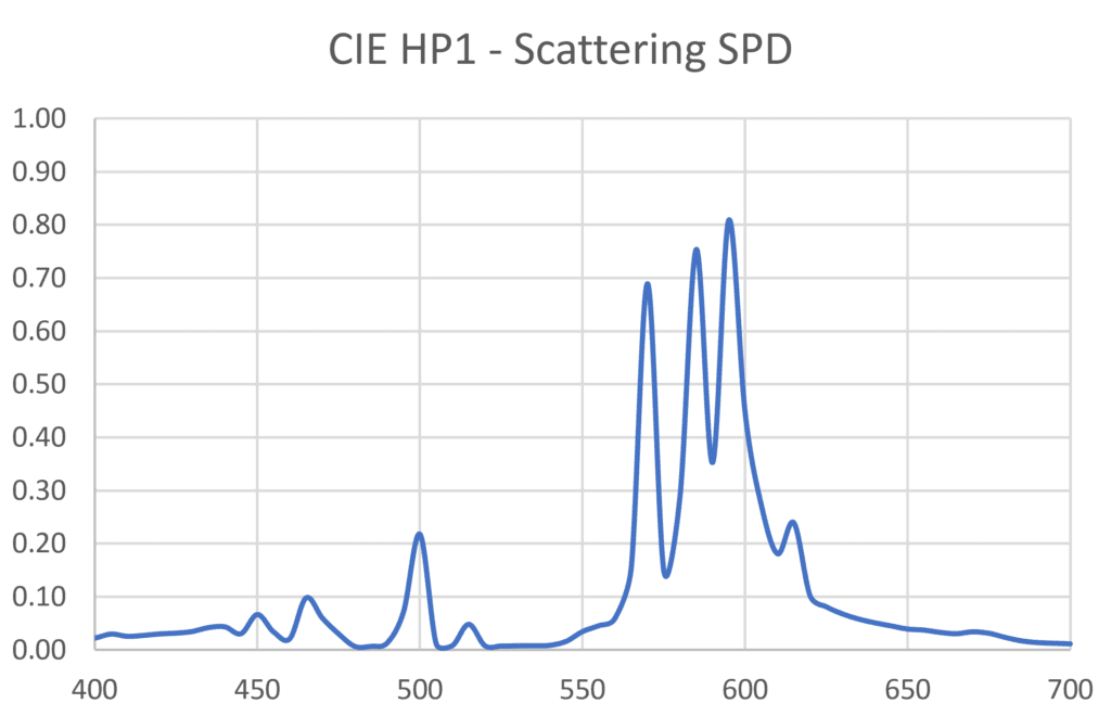
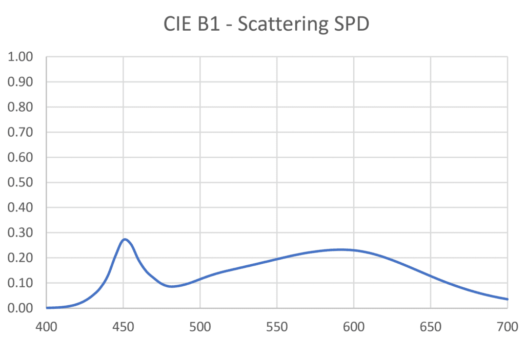
If we multiply the scaled light source SPDs by the atmospheric scattering on a per-wavelength basis, we obtain the scattering SPDs shown in Figure 7. These represent the spectrum of the sky glow contributed by the light sources. (There is also natural sky glow caused by airglow, zodiacal light, and scattered starlight, with a typical limiting magnitude of 21.)
Scotopic Vision
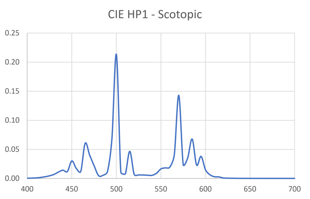
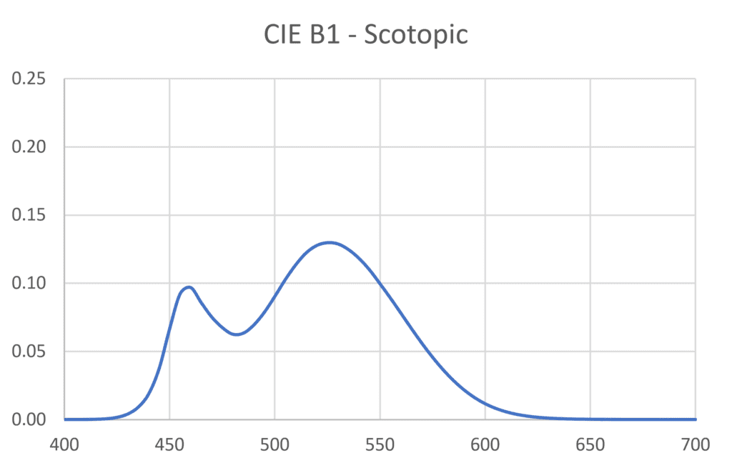
Under dark skies with fully dark-adapted eyes, the spectral response of our eyes is described by the scotopic efficiency function V′(λ), shown in Figure 4. We must therefore multiply each tabulated wavelength value of the scattering SPDs by the corresponding wavelength value of the scotopic efficiency function to obtain the scotopic SPDs shown in Figure 8.
If we sum the tabulated wavelength values of each scotopic SPD and multiply by a constant, we could calculate the contribution to sky luminance. This however is not our goal – we simply want to know the relative contribution to sky luminance due to the SPD of each light source. For any given light source, we therefore divide the sum of the tabulated values of its scotopic SPD by the sum of the tabulated values of the scotopic SPD of our baseline light source CIE HP1. This gives us the relative scotopic luminance values enumerated in Table 3.
| Light Source | Relative Scotopic Luminance |
| CIE HP1 | 1.00 |
| CIE HP2 | 1.98 |
| CIE HP3 | 2.64 |
| CIE HP4 | 3.20 |
| CIE HP5 | 3.64 |
| CIE B1 | 2.34 |
| CIE B2 | 2.60 |
| CIE B3 | 3.50 |
| CIE B4 | 3.82 |
| Generic 2200K | 1.53 |
| Generic PC Amber | 1.14 |
| Generic Amber | 0.32 |
Relative Limiting Magnitude
Finally, we need to convert the relative scotopic luminance values to relative limiting magnitude values using Pogson’s equation:
Mlimit = -2.5 log10(Lscotopic)
This equation accounts for our approximately logarithmic response to photometric intensity, and gives us the relative limiting magnitude values presented in Table 4.
| Light Source | Relative Sky Luminance |
| CIE HP1 (baseline) | 0.00 |
| CIE HP2 | -0.74 |
| CIE HP3 | -1.05 |
| CIE HP4 | -1.26 |
| CIE HP5 | -1.40 |
| CIE B1 | -0.92 |
| CIE B2 | -1.04 |
| CIE B3 | -1.36 |
| CIE B4 | -1.46 |
| Generic 2200K | -0.46 |
| Generic PC Amber | -0.14 |
| Generic Amber | +1.23 |
This then is the quantitative light pollution metric we have sought. The values are more usefully presented in Figure 9, where we can see at a glance how the different light sources compare.
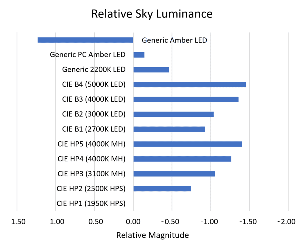
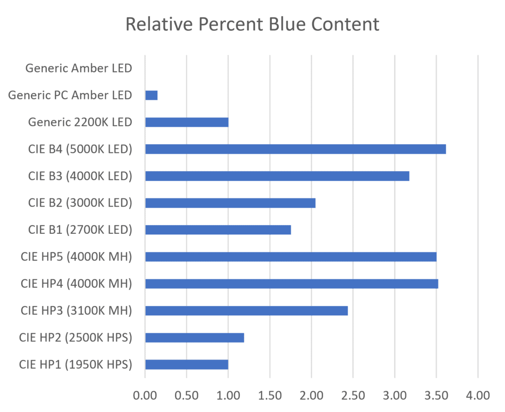
It is further interesting to compare these results to that of percent blue content for each light source, as shown in Figure 10 (with a cutoff wavelength of 520 nm). The ranking is the same as the relative sky luminance shown in Figure 9, but the quantitative differences can be misleading.
Metric Calculation
High-pressure sodium lamps from different manufacturers will likely have different SPDs, but the CIE HP1 lamp has the advantage of providing a standard baseline (i.e., a reference light source) for the proposed light pollution metric. With this, the calculation procedure for any target light source, present or future, consists of:
- Normalize the reference and target SPDs.
- Multiply SPDs by photopic efficiency function V(λ).
- Sum tabulated values of resultant photopic SPDs.
- Multiply photopic SPDs by sum divided by reference sum to produce scaled SPDs.
- Multiply scaled SPDs by atmospheric scattering function.
- Multiply scattering SPDs by scotopic efficiency function V′(λ).
- Sum tabulated values of resultant scotopic SPDs.
- Multiply scotopic SPDs by sum divided by reference sum.
- Calculate relative limiting magnitude.
Greenhouse Supplemental Lighting
Horticultural light pollution is a particular concern, as the light levels needed for crops within greenhouses at night can be on the order of one hundred to one thousand times those required for roadway and area lighting.
The photosynthetic photon flux output of horticultural luminaires is measured in micromoles per second rather than lumens, and the spectral output is expressed as a spectral quantum distribution (SQD) rather than a spectral power distribution (SPD). However, these details become unimportant when relative values are considered.
The equation to convert an SPD to an SQD is:
VQ(λ) = VP(λ) * λ * c
where VP(λ) is the SPD value at wavelength λ, VQ(λ) is its corresponding SQD value, and c is a constant. The value of the constant is not important, as the SQD will be normalized afterwards.
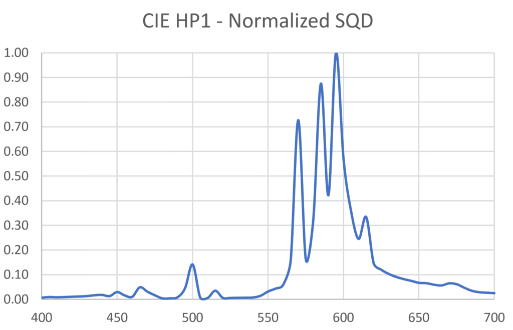
High-pressure sodium lamps have been a mainstay of supplemental electric lighting for greenhouses since the 1960s, so we can again use the CIE HP1 lamp as a baseline reference source. The SPD and corresponding SQD for this lamp are shown in Figure 11. (The two distributions are almost identical, apart from the smaller peak at 500 nm; this is not necessarily true for all SPDs.)

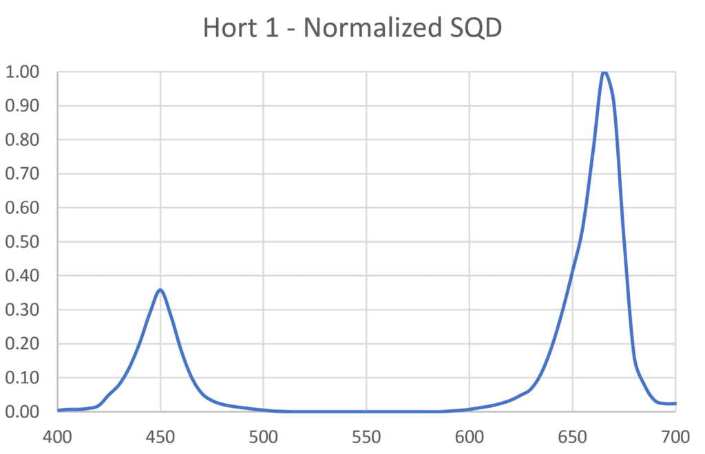
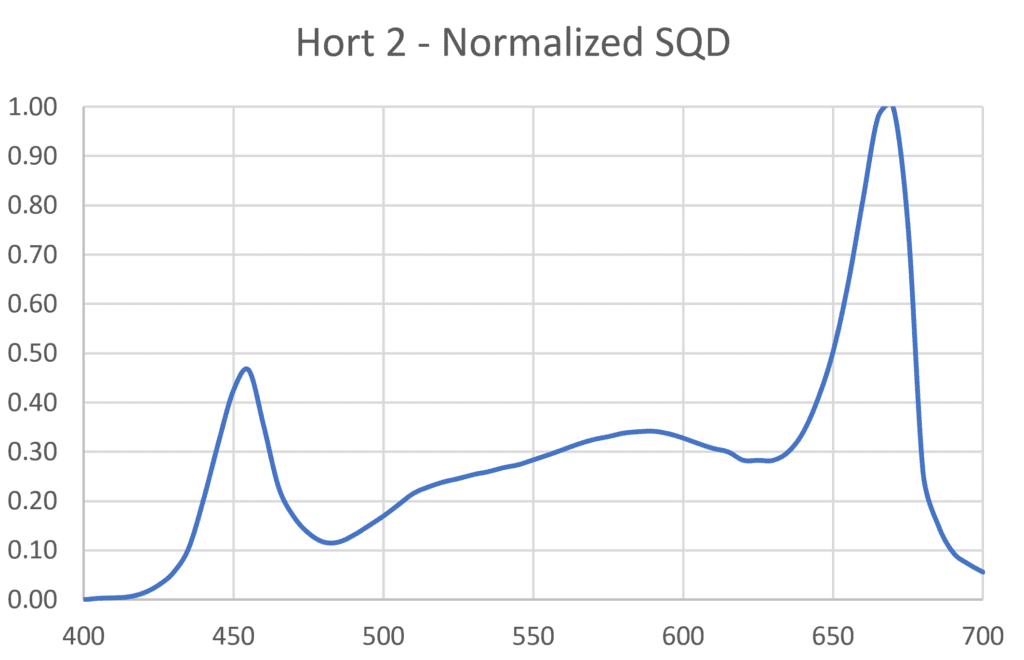
With this, we can consider two typical horticultural SQDs as shown in Figure 12. The luminaire labelled Hort 1 has 450 nm blue and 660 nm red LEDS designed to maximize photosynthesis, while the luminaire labelled Hort 2 includes phosphors that provide additional green light to benefit the plant growth and health.
The calculation procedure for horticultural luminaires is somewhat different:
- Convert reference SPD to normalized reference SQD.
- Sum tabulated values of normalized SQDs.
- Multiply normalized SQDs by sum divided by reference sum to produce target scaling factor.
- Convert target SQD to normalized SPD.
- Multiply target SPD by scaling factor.
- Multiply SPDs by atmospheric scattering function.
- Multiply scattering SPDs by scotopic efficiency function V′(λ).
- Sum tabulated values of resultant scotopic SPDs.
- Multiply scotopic SPDs by sum divided by reference sum.
- Calculate relative limiting magnitude.
Following this procedure, the relative limiting magnitude of the Hort 1 luminaire is +0.16 (i.e., slightly better than the baseline HPS lamp), while the relative limiting magnitude of the Hort 2 luminaire is -0.49 (i.e., about the same as a 2200K LED luminaire).
S/P Ratios
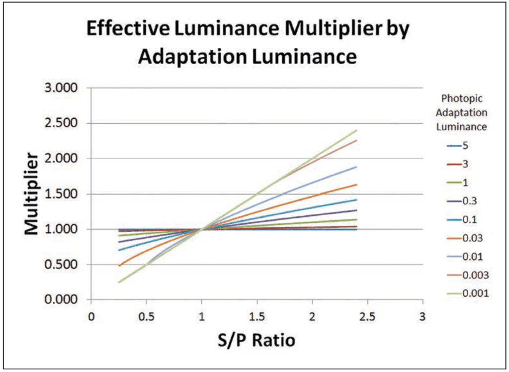
About a decade ago, there was considerable academic interest in mesopic vision, where the perceived (not measured) luminance of objects depends on the scotopic-to-photopic (S/P) ratio of the light source and the photopic adaptation (i.e., background) luminance. This resulted in effective luminance multipliers being recommended by CIE 191:2010, Recommended System for Mesopic Photometry Based on Visual Performance (CIE 2010), and IES TM-12-12, Spectral Effects of Lighting on Visual Performance at Mesopic Lighting Levels (IES 2012).
This concept was adopted by British Standard BS 5489-1, Code of Practice for the Design of Road Lighting, in 2013, but later mostly abandoned in the latest revision (BSI 2020). Today, it is recommended that the use of S/P ratios be discontinued when using white light sources with an CIE General Colour Rendering Index Ra greater than 70 (CIE 1995).
| Light Source | S/P Ratio |
| CIE HP1 (baseline) | 0.56 |
| CIE HP2 | 1.06 |
| CIE HP3 | 1.36 |
| CIE HP4 | 1.59 |
| CIE HP5 | 1.79 |
| CIE B1 | 1.21 |
| CIE B2 | 1.33 |
| CIE B3 | 1.72 |
| CIE B4 | 1.85 |
| Generic 2200K | 0.84 |
| Generic PC Amber | 0.71 |
| Generic Amber | 0.24 |
One of the reasons for this recommendation is that S/P ratios favor light sources with higher CCTs (Table 5). By ignoring mesopic lighting multipliers for “white” light sources, the use of high-CCT LED light sources is discouraged.
This would appear to complicate matters if CIE HP1 is taken as the baseline light source – it has an S/P ratio of 0.56 and a CRI Ra value of 24. However, the minimum recommended illuminance for pedestrian walkways in rural areas is about two lux (e.g., IES 2014). If we assume a typical diffuse ground reflectance of 15 percent, this means that the adaptation luminance is about 0.3 cd/m2. Referring to Figure 13 (and also to Annex A of IES TM-12-12), the effective luminance multiplier for CIE HP1 is about 0.94. In other words, the effective luminance multiplier for white light sources compared to CIE HP1 is at most an insignificant six percent. (Calculation results within ten percent of the target illuminance are considered to meet the design goal.)
Narrow amber, PC amber, and 2200K LED light sources are not “white,” as so the S/P ratios should, in accordance with BS 5489-1 recommendations, be applied. Again, however, we need to consider the minimum adaptation luminance of 0.3 cd/m2. This is off the chart of Annex A, which covers the range of 0.001 to 0.1 cd/m2. However, a reasonable extrapolation for the worst case of narrowband amber yields an effective luminance multiplier of 0.93.
Mesopic vision is also recognized by ANSI/IES RP-8-14, Roadway Lighting (IES 2014), which recommends that effective luminance multipliers “only be used to assess the luminances of off-road locations in applications for street lighting where the posted speed limit is 25 mph (40 km/h) or less” and “In cases where extraneous light sources or surroundings increase adaptation levels significantly above those of the pavement luminance, these factors are not appropriate.”
For all practical purposes in outdoor nighttime lighting applications then, effective luminance multipliers based on the S/P ratio of the light source do not apply.
Conclusion
The primary advantages of the proposed metric are that:
- It is based on a reasonable model of the physical and visual processes that result in our perception of light pollution;
- It relies on a straightforward calculation procedure; and
- The metric is simple enough for a schoolchild to explain.
To further explain the third point, the schoolchild does not need to explain how the metric is calculated. Rather, it becomes as simple as saying, “Bigger (negative) numbers means that we can see fewer stars in the night sky.” This is on par with saying, “Miles per gallon (MPG) is the distance that a car can travel on a gallon of fuel.” Explaining how this metric is calculated is an entirely different issue.
Some caution, however, should be taken in applying the metric to outdoor lighting design. For most applications, a difference of one-half magnitude is significant. Thus, there should be a good reason for specifying, for example, 4000K LED lighting rather than 3000K as recommended by the International Dark-Sky Association. (One argument might be that color discrimination is important.) The difference between the two may be only one-third magnitude, but it is still noticeable visually.
On the other hand, the difference between 2700K and 3000K LED lighting is only 0.08 magnitudes (based on the CIE SPDs). It would be difficult to argue that this is significant for any practical application if – a very big if – astronomical light pollution for visual star-gazing is the only design criterion. In general, lighting designers will need to take into consideration other factors, such as color discrimination for drivers and pedestrians, the effect of short-wavelength (“blue”) light at night on insects, birds, amphibians, fish, and mammals, color preferences of homeowners on residential and commercial streets, light-source temperature dependencies (especially narrowband amber LEDs), luminaire efficacy, capital and operating costs, and more.
While spectral power distribution data are rarely available from luminaire manufacturers in tabular form, this is not a particular problem. The light source SPDs published in CIE (2018) are more than adequate in calculating light pollution metrics for different classes of light sources. The point of this metric is not to provide immutable guidelines for lighting designers, but to provide quantifiable values on which to base these decisions.
Acknowledgements
The author thanks Eric Bretschneider and David Woodward for their useful and productive review comments.
References
Aubé, M. 2015. “Physical Behaviour of Anthropogenic Light Propagation into the Nocturnal Environment,” Philosophical Transactions of the Royal Society B 370(1667):20140117.
BSI. 2020. BS 5489-1:2020, Code of Practice for the Design of Road Lighting, Part 1 – Lighting of Road and Public Amenity Areas. British Standards Institution.
CIE 1995. CIE 13.3-1995, Method for Measuring and Specifying Colour Rendering Properties of Light Sources. Vienna, Austria: CIE Central Bureau.
CIE. 2010. CIE 191:2010, Recommended System for Mesopic Photometry Based on Visual Performance. Vienna, Austria: CIE Central Bureau.
CIE. 2018. CIE 015:2018, Colorimetry, Fourth Edition. Vienna, Austria: CIE Central Bureau.
IES. 2012. IES TM-12-12, Spectral Effects of Lighting on Visual Performance at Mesopic Lighting Levels. New York, NY: Illuminating Engineering Society.
IES. 2014. ANSI/IES RP-8-14, Roadway Lighting. New York, NY: Illuminating Engineering Society.
0 Comments
Trackbacks/Pingbacks