
This is a preprint of a paper presented by the author at the International Society for Horticultural Lighting (ISHS)’s GreenSys 2019 conference in Angers, France in June 2019, and scheduled for publication in Acta Horticulturae .
Abstract
Recent advances in LED-based luminaire design have enabled greenhouse operators to temporally control both the photon flux density (PFD) and spectral irradiance incident upon the plant canopy. However, it is difficult to predict the performance and benefits of these luminaires without knowledge of the time-varying PFD and spectral irradiance due to daylight. We have addressed this problem with the development of horticultural lighting design software that incorporates validated climate-based annual daylighting calculations, physically-based modelling of glazing and light diffusion materials, modelling of spectral reflectance from greenhouse crops and surrounding surfaces, and accurate simulation of optical radiation distribution within the greenhouses from direct sunlight, diffuse daylight, and supplemental electric light sources. These measurements can be used to determine daylight availability, monthly Daily Light Integrals, automated shade and energy curtain deployment schedules, and projected electrical energy costs, all in advance of building the physical structures.
Introduction
Since their commercial introduction in 1964, high-pressure sodium (HPS) lamps have been a mainstay of supplemental electric lighting in greenhouses. With their fixed light outputs and spectral power distributions (SPDs), however, there has been little incentive or opportunity for commercial greenhouse operators with experiment with different “light recipes” for optimum plant growth and health. Rather, the luminaires are typically turned on at dusk and operated until the desired Daily Light Integral (DLI) for the crop or ornamental plats is achieved.
The introduction of light-emitting diodes (LEDs) for horticultural lighting has completely changed this situation. Many luminaire manufacturers are now offering products with separate SPD settings for promoting vegetative growth and blooming. Some manufacturers are going further by including, in addition to the ubiquitous 450 nm blue and 660 nm red LEDs, ultraviolet-A, green and “white light” LEDs with different correlated color temperatures (CCTs), and also 735 nm far-red LEDs. Going further still, a few products can be dimmed in response to inputs from daylight sensors, and it likely that future products will enable computer control of their SPDs beyond simple “veg” and “bloom” settings.
Together, these studies indicate that successful light recipes may involve daily dynamic changes in both the photon flux density (PFD) and SPDs delivered to crops and ornamentals in greenhouses. However, there is a problem. Most of these studies have been conducted in controlled environment growth chambers. It is often difficult to translate such laboratory research to greenhouse environments (e.g., Annunziata et al., 2017). Even if light recipes for a given crop or ornamental are developed in a research greenhouse, it is difficult to ensure that all of the requirements are met in commercial greenhouses. Certainly, such simple metrics as DLI are not enough.
GREENHOUSE MODELLING
Modelling a greenhouse begins with its most important element: glazing.
Glazing
For the purposes of daylighting, glazing materials have three important optical properties:
Fresnel transmittance.
The optical transmittance of transparent glass and rigid plastic panels (collectively dielectric materials) depends on the angle of incidence q of the incoming light (Figure 1). At normal incidence (i.e., q = 0 degrees), each surface reflects about 4 percent of the light. A single pane has two surfaces, and so the maximum possible transmittance is 92 percent. Double-pane and triple-pane insulated glass panels correspondingly have maximum possible transmittances of 85 percent and 78 percent respectively
What is more important is that the transmittance decreases with increasing angle of incidence, as determined by the “Fresnel equations” (e.g., Ashdown, 2019). This is clearly evident when reflections of the Sun from windows are viewed at grazing angles. Anti-reflection (AR) coatings can improve the transmittance somewhat at normal incidence, but the Fresnel transmittance still dominates at large incidence angles.
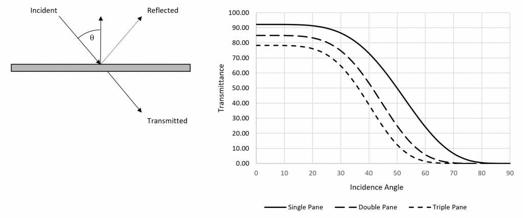
Figure 1. The transmittance of transparent glazing depends on the angle of incidence q and the number of panes.
It is also important to note that Figure 1 applies to daylight with a specific angle of incidence. Looking at the graph, it is evident that the transmittance of direct sunlight through the greenhouse glazing panels will depend on the solar position (azimuth and altitude), the building orientation, and the roof panel slope. The solar position varies throughout the day and year, of course, and so any transmittance calculations need to be performed on an hourly basis.
What is less evident is that daylight is comprised of both direct sunlight and diffuse daylight. On a clear summer day at noon, the ratio of direct sunlight to diffuse daylight incident on a surface facing the sun may be 20:1 or so; on an overcast day, there is no direct sunlight. In addition, the amount of daylight diffusely reflected from the ground and incident on vertical surfaces is typically 20 percent or so. The graph shown in Figure 1 is therefore instructive but not useful for calculation purposes.
Diffusion.
There is growing evidence that plants use diffuse light more effectively than direct sunlight (e.g., Li and Yang, 2015). Particularly for shade-tolerant plants, translucent glazing results in more even spatial distribution of photosynthetic photon flux (PPFD) within the greenhouse, and also reduces its temporal variation on clear days.
Of course, the analytic modelling method for diffusion materials can also be used to represent greenhouse shade cloth, paint materials, and condensation on otherwise non-diffusing glazing.
Spectral transmittance.
The spectral range of photobiologically active radiation (PBAR) is generally assumed to be 280 nm to 800 nm (ASABE, 2017). This includes ultraviolet-B (280 nm to 315 nm) and ultraviolet-A (315 nm to 400 nm). However, soda-lime glass is opaque to ultraviolet radiation below approximately 320 nm, and so UV-B radiation, while shown to be beneficial to field-grown plants, is not a consideration in greenhouses. Similarly, low-density polyethylene (LDPE) used as an agricultural film for polytunnels, is opaque below 350 nm (Cadena and Acosta, 2014), while polycarbonate is opaque below 390 nm.
Given this, it is reasonable to model spectral irradiance inside greenhouses and polytunnels from 350 nm to 800 nm, where the spectral transmittance of soda-lime glass, LDPE, and polycarbonate is basically constant.
Greenhouse Structure
For most greenhouse designs, the purpose of the greenhouse structure is to support the glazing and possibly fan housings and motorized shades. From the perspective of climate-based daylight modelling, it is the size, position, and orientation of the glazing panels (or film for polytunnels) that is most important.
While there are many custom greenhouse designs, almost all commercial greenhouses can be classified as having arch, Gothic, Venlo, or sawtooth roofs, while polytunnels can be classified as having either arch or Gothic hoops (Figure 2).
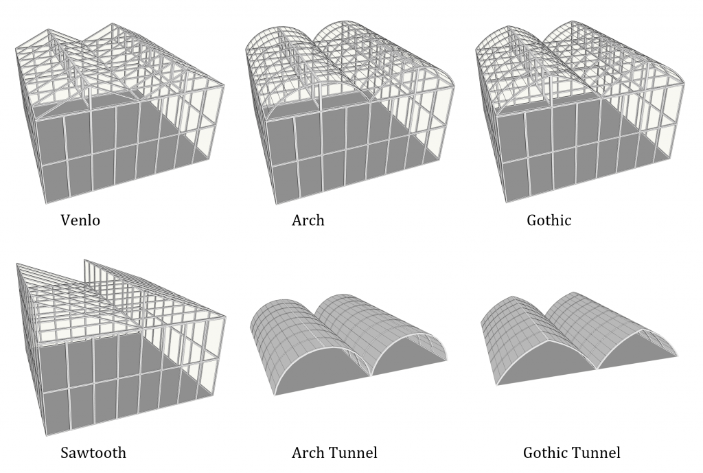
Figure 2. Four different greenhouse roof styles and two different polytunnel hoop styles determine how direct sunlight and diffuse daylight are transmitted through the roof panels.
While not directly related to daylight modelling, it would clearly be a time-consuming exercise for a typical user (for example, a greenhouse or horticultural luminaire manufacturer) to design and model an entire greenhouse with all the side posts, rafters, support columns, purlins, and cross ties. Fortunately, the simplicity of the framework makes it possible to use parametric design techniques, where the software generates the entire greenhouse structure from a few user-specified parameters. This can include the dimensions and spacing of tables, the placement of horticultural luminaires as supplemental electric lighting, and the specification of motorized shades.
A computer-aided drafting (CAD) model as shown in Figure 3 and needed for the daylighting calculations can be generated from the user-specified parameters in a fraction of a second. Due to the modular nature of greenhouses, even greenhouses as large as hundreds of thousands of square meters can be generated in the same amount of time.
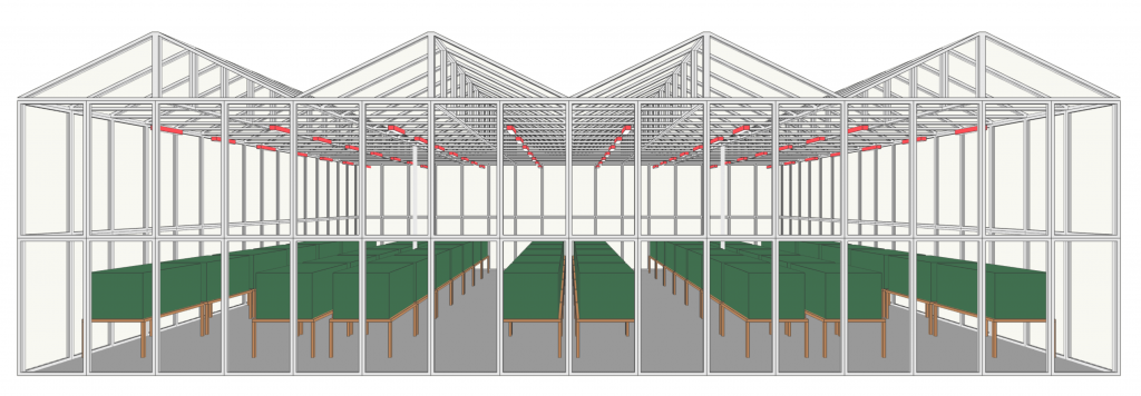
Figure 3. Automatically-generated CAD model of a Venlo greenhouse.
Horticultural Luminaires
For over a century, architectural luminaires have been modeled as point light sources with angular luminous intensity distributions (Figure 4). For more than thirty years, the laboratory measurements have been reported using formatted text files that lighting design software programs can read.
To address this issue, an international standard was developed with specific support for horticultural lighting. Currently published in the United States (IES, 2018) and Italy (UNI, 2019), it is being developed for publication as a worldwide ISO standard. Its features include:
- Photon intensity distribution (measured in µmol ´ sr-1 ´ sec-1)
- Total photon flux (measured in µmol ´ sec-1)
- Spectral power distribution (measured in watts ´ nm-1)
- Channel multiplier
If the luminaire allows the LED color intensities to be individually controlled, these can be represented by a “channel multiplier” for each color that represents the channel dimmer setting when the luminaire’s optical characteristics were measured.
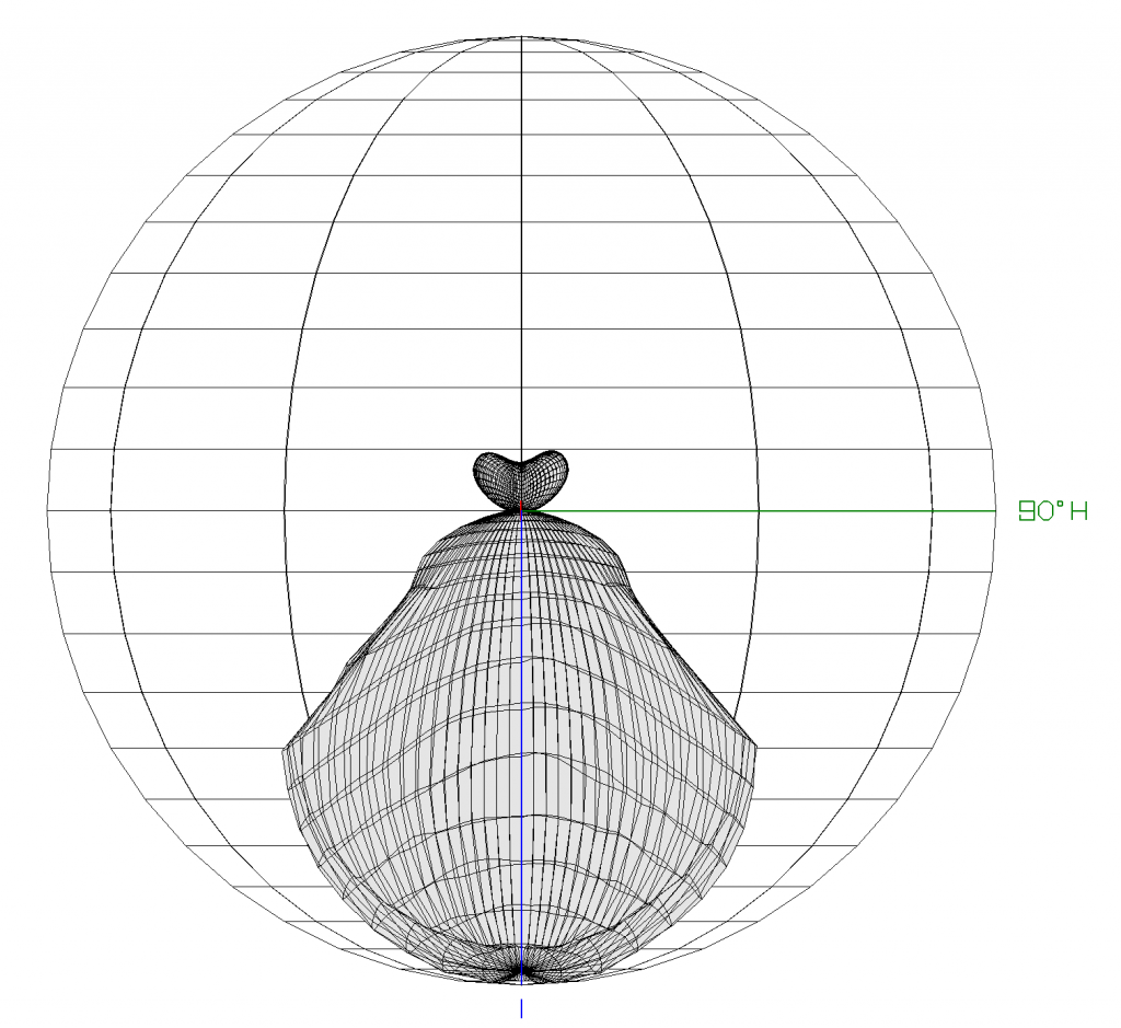
Figure 4. Luminaire photon intensity distribution.
Horticultural luminaire manufacturers currently report photosynthetic photon intensity distributions (or a multiplier to convert from lumens to photon flux). However, future light recipes will require more information than this. Accordingly, the spectral range is specified for the photon measurements (minimum and maximum wavelengths) so that it is possible to represent ultraviolet (280 nm – 400 nm), photosynthetic (400 nm – 700 nm), and far-red (700 nm – 800 nm) photon intensity and flux values (ASABE, 2017).
Weather Data
To calculate the daylight incident on a greenhouse, the software needs to know the building’s latitude, longitude, and compass (orientation). With this, it is possible to locate the nearest weather station for which a Typical Meteorological Year (TMY) weather dataset is available. One example is the collection of EnergyPlus TMY3 datasets, representing over 2,500 locations worldwide, although there are other datasets available that have been derived from combinations of historical weather data and weather satellite observations.
Virtual PAR Sensors
To measure the spatial distribution of PPFD on the plant canopy in the greenhouse, it is necessary to specify a horizontal array of virtual PAR (quantum) sensors. Each sensor will then receive direct sunlight, diffuse daylight, and direct photon flux from the luminaires (if any).
There are no restrictions on the position and orientation of the PAR sensors, so they could also for example be placed between the plant rows and oriented to measure vertical rather than horizontal photon flux, including that reflected from the floor and plant leaves.
Daylight Calculations
Once the greenhouse has been modeled and a weather dataset appropriate for the location obtained, the climate-based annual daylight calculations can be performed. Each weather dataset typically has 8,760 hourly records, so there are 4,380 different daylighting scenarios that must be considered.
The daylight calculations occur in two phases. In the first phase, the daylight incident on the exterior of the building is determined. This includes determining:
- The solar position (altitude and azimuth) for a given time and date;
- The direct solar irradiance;
- The spatial distribution of diffuse daylight radiance on the sky dome;
- The daylight diffusely reflected from the ground; and
- The daylight SPD.
where the spatial distribution of the diffuse daylight is calculated in accordance with the industry-standard Perez sky model (Perez et al., 1993). The daylight calculation algorithms are detailed elsewhere (Ashdown, 2017).
Daylight SPD
Both direct sunlight and diffuse daylight have SPDs that closely resemble that of a black-body radiator, and so they can be uniquely described by their color temperature, expressed in kelvins (K). Direct sunlight has a color temperature of approximately 5500K, while that of clear blue sky typically ranges from approximately 7500K to 15,000K.
The SPD of daylight with color temperatures greater than 4000K can be calculated using the equations presented in CIE 15:4, Colorimetry (CIE, 2004). For example, the combination of direct sunlight and diffuse daylight on a clear day has a color temperature of approximately 6500K (which is the same white color as a computer display); the corresponding SPD is shown in Figure 6.
For overcast skies, clouds are spectrally neutral and so scatter daylight without changing its SPD. Consequently, a typical overcast sky has a color temperature between 6000K and 6600K (Lee and Hernández-Andréz, 2006). Given this, it is reasonable to assume a color temperature of 5500K for direct sunlight, 10,000K for clear blue sky, and 6500K for overcast sky.
Radiosity calculations
The second phase of the daylight and electric lighting calculations determine the spatial distribution and temporal changes in PPFD within the greenhouse. These calculations use a version of radiative flux transfer equations referred to as the radiosity method, and have been detailed elsewhere (e.g., Ashdown, 1994). Of significance for horticultural lighting design is that even though some 4,380 hourly daylight scenarios must be calculated, the calculation times are on the order of a few seconds to a few minutes, depending on the size of the greenhouse (Ashdown, 2018a).
Automated Shades
Automated shades are a common approach to limit the amount of direct sunlight incident upon the plant canopy. Given this, designated glazing panels in the greenhouse models can be modelled as being both transparent and diffusing (or, for energy curtains, opaque). This has no effect on the daylight or electric lighting calculation times, but it does mean that after the calculations have been completed, the spatial distribution of PPFD within the greenhouse can be accessed on a per-hour basis afterwards with the shades either open or closed.
Virtual Spectroradiometer
Architectural lighting design software models light sources as being “white,” and all surface colors as being combinations of red, green, and blue components. This works well for both lighting calculations and architectural visualizations, but it means that the daylight and luminaire SPDs cannot be represented. (They could, but it would require that the spectral reflectance distributions of all surfaces would need to be known, and greatly increasing the calculation times and memory requirements.)
Fortunately, there are mathematical techniques borrowed from remote satellite imaging that obviate the need for spectral reflectance distributions (e.g., Fairman and Brill, 2004). Instead, given only the red, green and blue components of a color, it is possible to reconstruct a physically plausible SPD. With this, it is possible to implement a virtual spectroradiometer that can be positioned and oriented anywhere in the greenhouse after the lighting calculations have been completed.
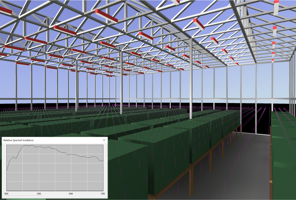
Figure 5. Virtual spectroradiometer measuring daylight SPD inside a greenhouse.
RESULTS ANALYSIS
Once the daylight and electric lighting calculations have been completed, the most obvious analyses include calculating the predicted monthly DLIs and predicted electrical energy costs for the proposed buildings. However, new tools introduce new opportunities, and CBDM for greenhouses is no exception.
As one example, shade fabrics are available with a wide range of absorption and diffusion characteristics. By modelling different fabrics in software, it is possible to determine which will offer the best performance for different crops, taking into account the monthly DLIs and peak PPFDs rather than simply calculating an example time and date.
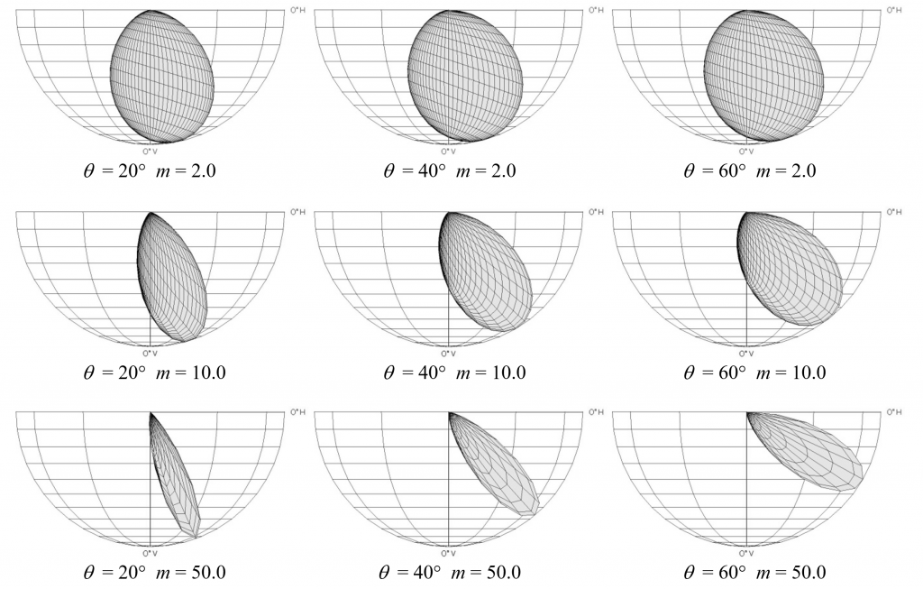
Figure 6. Analytic bidirectional scattering distribution function (BSDF) of diffiuion material.
Automated shades and energy curtains are another example. The calculation results can be used to develop automatic shade deployment schedules in response to changing weather conditions. It may be, for example, that the shades are ineffective – something that can be determined during the design phase rather than after construction.
Yet another example is light pollution. Increasing attention is being paid to the negative aspects of greenhouse lighting at night – light trespass onto neighbouring residential properties, increased sky glow (especially on overcast nights with low cloud cover), and ecological disruption for both animals and plants. Greenhouse lighting design software can be used to model and predict these problems. (As one particular example, roof-mounted energy curtains can potentially result in a 20 percent or more reduction in electrical operating costs due to the light being reflected back down onto the plant canopy.)
Finally, a virtual spectroradiometer is the ideal tool for predicting the spectral distribution of photon flux anywhere in the greenhouse. As light recipes become more sophisticated, such a tool becomes increasingly valuable.
CONCLUSIONS
As stated in the introduction, the goal of this paper has been to report on the development of climate-based daylight modelling software specifically for greenhouses and polytunnels with optional supplemental electric lighting. The focus has been on the horticultural aspects of the software from a user’s perspective, with as few references to computer science and related topics as possible. To do otherwise would have required at least several textbooks worth of material.
The real goal of this paper has been to introduce what is basically a new tool for greenhouse designers, and to explore the issues that it addresses. This paper will hopefully provide the foundation for further conversations between horticulturalists and software developers responsible for such tools.
ACKNOWLEDGEMENTS
The author wishes to thank Peter Socha for his assistance in the research for this paper.
Literature cited
Annunziata, M.G., Apelt, F., Carillo, P., Krause, U., Feil, R., Mengin, V., Lauxmann, M.A., Köhl, K., Nikoloski, Z., Stitt, M., et al. J.E. (2017.) Getting back to nature: a reality check for experiments in controlled environments. J. Exp. Bot. 68 (16), 4463–4477 http://dx.doi.org/10.1093/jxb/erx220.
ASABE. (2017.) ANSI/ASABE S640 JUL2017, Quantities and Units of Electromagnetic Radiation for Plants (Photosynthetic Organisms). (St. Joseph, MI: American Society of Agricultural and Biological Engineers.)
Ashdown, I. (1994.) Radiosity: A Programmer’s Perspective. (New York, NY: John Wiley & Sons.)
Ashdown, I. (2016.) Climate-based daylight modeling: from theory to practice. http://dx.doi.org/10.13140/RG.2.2.19325.20969.
Ashdown, I. (2017.) Analytic BSDF modeling for daylight design. Paper presented at: IES 2017 Annual Conference, Portland, OR. (New York, NY: Illuminating Engineering Society).
Ashdown, I. (2018a.) LICASO and DAYSIM: a comparison. http://dx.doi.org/10.13140/RG.2.2.25669.09441.
Ashdown, I. (2018b.) Far-red lighting and the phytochromes. Maximum Yield 20 (7), 60-66 (October).
Ashdown, I. (2019.) Light transmittance through greenhouse glazing. Maximum Yield 21 (3), 50-51 (March).
Cadena., C., and Acosta, D. (2014.) Effects of solar UV radiation on materials used in agricultural industry in Salta, Argentina: study and characterization. J. Mat. Sci. Chem. Eng. 2, 1-14 http://dx.doi.org/10.4236/msce.2014.24001.
CIE. (2004.) Colorimetry, Third Edition. CIE Technical Report 15:2004. (Vienna, Austria: Commission Internationale de l’Eclairage.)
Craig, D.S., and Runkle, E.S. (2013.) A moderate to high red to far-red light ratio from light-emitting diodes controls flowering of short-day plants. J. Am. Soc. Hortic. Sci. 138 (3), 167–172 http://dx.doi.org/10.21273/JASHS.138.3.167.
Demotes-Mainard, S., Péron, T., Corot, A., Bertheloot, J., Gourrierec, J., Pelleschi-Travier, S., Crespel, L., Morel, P., Huché-Thélier, L., Boumaza, R., et al. (2016.) Plant responses to red and far-red lights, applications in horticulture. Env. Exp. Bot. 121, 4–21 http://dx.doi.org/10.1016/j.envexpbot.2015.05.010.
Fairman, H.S., and Brill, M.H. (2004.) The Principal Components of Reflectances. Color Res. App. 29 (2), 104-110 http://dx.doi/10.1002/col.10230.
Giancomelli, G.A. (2011.) Greenhouse Glazing. In Ball Redbook Vol. 1., 18th edn, C. Beytes, ed. (Chicago, IL: Ball Publishing), p.23-41.
Hanyu, H., and Shoji, K.. (2002.) Acceleration of growth in spinach by short-term exposure to red and blue light at the beginning and at the end of the daily dark period. Acta Hortic. 580, 145-150 http://dx.doi.org/10.17660/ActaHortic.2002.580.17.
Huché-Thélier, L., Crespel, L., Gourrierec, J., Morel, P., Sakr, S., and Leduc, N. (2016.) Light signaling and plant responses to blue and UV radiations – perspectives for applications in horticulture. Env. Exp. Bot. 121, 22–38 http://dx.doi.org/10.1016/j.envexpbot.2015.06.009.
IES. (2018.) ANSI/IES TM-33-2018, Standard Format for the Electronic Transfer of Luminaire Optical Data. (New Yok, NY: Illuminating Engineering Society.)
Lee, R.L., and Hernández-Andrés, J. (2006.) Colour of the Daytime Overcast Sky. App. Optics 44 (27), 5712-5722 http://dx.doi.org/10.1364/AO.44.005712.
Li, T., and Yang, Q. (2015.) Advantages of diffuse light for horticultural production and perspectives for further research. Front. Plant Sci. http://dx.doi.org/10.3389/fpls.2015.00704.
Liu, H., Fu, Y., Hu, D., Yu, J. and Liu, H. (2018.) Effect of green, yellow and purple radiation on biomass, photosynthesis, morphology and soluble sugar content of leafy lettuce via spectral wavebands ‘knock out’. Sci. Hortic. 236, 10–17 http://dx.doi.org/10.1016/j.scienta.2018.03.027.
Perez, R., Seals, R., and Michalsky, J. (1993.) All-weather model for sky luminance distribution – preliminary configuration and validation. Solar Energy 50 (3), 235-245. http:///dx.doi.org/10.1016.0038-092X(93)90017-I.
Ponce, P., Molina, A., Cepeda, P., Lugo, E, and MacCleery, B.. (2015.) Greenhouse Design and Control. (Leiden, The Netherlands: CRC Press/Balkema.)
Seaton D.D., Toledo-Ortiz, G., Ganpudi, A., Kubota, A, Imaizumi, T., and Halliday, K.J. (2018.) Dawn and photoperiod sensing by phytochrome A,”. PNAS 115 (4), 10523–10528 http://dx.doi.org/10.1073/pnas.1803398115.
Song, Y.H., Kubota, A., Kwon, M.S., Covington, M.F., Lee, N., Taagen, E.R., Cintrón, D.L., Hwang, D.Y., Akiyama, R., Hodge, S.K., et al. (2018.) Molecular basis of flowering under natural long-day conditions in Arabidopsis. Nature Plants 4, 824-835 http://dx.doi.org/10.1038/s41477-018-0253-3.
Tregenza, P., and M. Wilson. (2015.) Daylighting: Architecture and Lighting Design. (London, UK: Routledge.)
UNI. (2019. UNI 11733:2019, Luce e illuminazione – specifiche per un formato di interscambio dati fotometrici e spettrometrici degli apparecchi di illuminazione e delle lampade. store.uni.com.
Verdaguer, D., Jansen, M.A.K., Llorens, L., Morales, L.O., and Neugart, S.. (2017.) UV-A radiation effects on higher plants: exploring the known unknown. Plant Sci. 255, 72–81 http://dx.doi.org/10.1016/j.plantsci.2016.11.014.
Wang, Y., and Folta, K.M. (2013.) Contributions of green light to plant growth and development. Am. J. Bot. 100 (1), 70–78 http://dx.doi.org/10.3732/ajb.1200354.
Wargent, J.J., Nelson, B.W.C., McGhie, T.K., and Barnes, P.W. (2015.) Acclimation to UV-B radiation and visible light in Lactuca sativa involves up-regulation of photosynthetic performance and orchestration of metabolome-wide responses. Plant, Cell Env. 38 (5), 929–940 http://dx.doi.org/10.1111/pce.12392.
Wargent, J.J. (2016.) UV LEDs in horticulture: from biology to application. Acta Hortic. 1134, 25–32 http://dx.doi.org/10.17660/ActaHortic.2016.1134.4.
0 Comments